Details¶

[This section is not meant to be a gentle introduction to lattices; it exists mainly to review the conventions used throughout the Bravais.jl codebase.]

The direct Bravais lattice¶

A Bravais lattice in $D$ dimensions is defined, given some “primitive vectors” $\mathbf{a}_i$ , to be all points $\mathbf{R} = \sum_{i=1}^D n_i \mathbf{a}_i$ where each $n_i \in \mathbb{Z}$ . (There is one primitive vector for each dimension in which the lattice extends.)

We cannot address (or store information about) an infinite number of points on a computer, so instead we choose a finite number of contiguous points from our infinite lattice, and label them as the points we will consider. If we wish to emulate a system without boundary and maintain the translation symmetry of the lattice, we will implement “periodic boundary conditions” (PBC, also known as Born-von Karman boundary conditions) in all directions. Another option is to implement fully open boundary conditions (OBC), in which case the lattice is simply truncated beyond the points of the finite lattice. Yet another option is to have OBC in some dimensions and PBC in others; one example of this is cylindrical boundary conditions in a 2D system.

Let’s get a bit more mathmatical. Given positive integers $N_1, \ldots, N_D$ along with the primitive vectors $\mathbf{a}_i$ , we define a finite lattice with $N_\mathrm{tot}=\prod_{i=1}^D N_i$ sites, each site given by $\mathbf{r}_\alpha = \sum_{i=1}^D n_i \mathbf{a}_i$ where $n_i \in \mathbb{Z}_{N_i}$ and $\alpha = 1, \ldots, N_\mathrm{tot}$ . (We will refer to $\alpha$ as the “index” of the site, and $(n_1, \ldots, n_D)$ as the “site label.”)

At this point, the finite lattice only represents a subset of the original lattice sites. For the case of periodic boundary conditions, we would like to repeat our “finite” lattice, tiling it throughout the lattice such that every site of our original infinite lattice is represented by some site on our finite lattice.

We define vectors $\mathbf{A}_1, \ldots, \mathbf{A}_D$ , each of which is some linear combination of the primitive vectors, such that each site on the infinite lattice can be written uniquely as $\mathbf{R} = \mathbf{r}_\alpha + \sum_{i=1}^D \tilde{N}_i \mathbf{A}_i$ , where $\tilde{N}_i \in \mathbb{Z}$ . There will often (particularly for $d>1$ ) be infinitely many different ways of choosing these vectors, some of which will result in “helical” boundary conditions (in which translating the length of the lattice in one dimension also results in an offset in one or more other dimensions).

Note

On an infinite lattice, there are many possible ways of choosing the primitive vectors, and they are all equivalent to each other. On a finite lattice, however, this is no longer the case. The choice of primitive vectors will dictate how the points of the finite lattice are arranged.

The reciprocal lattice¶

The reciprocal lattice of a Bravais lattice is defined as all wave vectors $\mathbf{K}$ satisfying $e^{i\mathbf{K}\cdot\mathbf{R}}=1$ for all points $\mathbf{R}$ in the infinite Bravais lattice. In other words, we require $\mathbf{K} \cdot \mathbf{R} = 2\pi M$ for some $M \in \mathbb{Z}$ . This can best be achieved by choosing the reciprocal lattice’s primitive vectors $\mathbf{b}_j$ such that $\mathbf{a}_i \cdot \mathbf{b}_j = 2\pi \delta_{ij}$ . Then each $\mathbf{K}$ can be written as $\mathbf{K} = \sum_{j=1}^D m_j \mathbf{b}_j$ with $m_j \in \mathbb{Z}$ . This gives $\mathbf{K} \cdot \mathbf{R} = \sum_{i=1}^D\sum_{j=1}^D n_i m_j \, \mathbf{a}_i \cdot \mathbf{b}_j = 2\pi \sum_{i=1}^D m_i n_i$ , which will always satisfy the original condition $e^{i\mathbf{K}\cdot\mathbf{R}}=1$ . (For more details, see e.g. Ashcroft and Mermin pages 86-87.)

It is worth noting that the reciprocal of the reciprocal lattice is the direct lattice itself.

Allowed momenta¶

We will begin by studying the case in which the boundary conditions in each direction are periodic/twisted [1]. With periodic/twisted boundary conditions on a finite lattice, only certain momenta are possible in the system. After exploring the case of fully periodic/twisted boundary conditions, we will extend our reasoning to include the (somewhat simpler) case in which one or all dimensions have open boundary conditions.

Bloch’s theorem says given a periodic system, the eigenstates of any Hamiltonian can be chosen such that each $\psi$ is associated with a wave vector $\mathbf{k}$ such that $\psi(\mathbf{r} + \mathbf{R}) = e^{i\mathbf{k} \cdot \mathbf{R}}\psi(\mathbf{r})$ for every $\mathbf{R}$ in the lattice [2]. Our goal in the following is to determine, given some boundary conditions on a finite lattice, what wave vectors $\mathbf{k}$ are allowed.

For a Bravais lattice, there will be as many allowed momenta as there are points on the finite lattice assuming PBC in each direction. Typically, allowed momenta are given by points within the first Brillouin Zone (BZ). We want to uniquely label the allowed momenta, but for simplicity we will label them systematically without the requirement that they be in the first Brillouin Zone.

We define the “twist” values $\eta_i$ such that

$\psi(\mathbf{r} + \mathbf{A}_i) = e^{2\pi i\eta_i}\psi(\mathbf{r})$

for all $i$ . (For a system without any twisted boundary conditions, $\eta_i=0\ \forall i$ .) We can combine our knowledge that $\mathbf{A}_i$ is in the lattice with Bloch’s theorem to give $e^{i\mathbf{k} \cdot \mathbf{A}_i}\psi(\mathbf{r}) = e^{2\pi i\eta_i}\psi(\mathbf{r})$ , or equivalently $e^{i\left[ \mathbf{k} \cdot \mathbf{A}_i - 2\pi\eta_i \right]} = 1$ , for all $i$ .

We know that the $\mathbf{A}_i$ ‘s must be linear combinations of the primitive vectors, so we can write them as $\mathbf{A}_i = \sum_{j=1}^D M_{ij} \mathbf{a}_j$ , where each $M_{ij}$ is an integer. (For periodic/twisted boundary conditions, our diagonal elements must be $M_{ii} = N_i$ , the lattice extent in each direction. We will see later that for any dimension $i$ in which we have open boundary conditions, we instead have $M_{ii} = 0$ .) We will also write our wave vector in terms of fractions of the reciprocal lattice’s basis vectors: $\mathbf{k} = \sum_{h=1}^D x_h \mathbf{b}_h$ . Then,

$\mathbf{k} \cdot \mathbf{A}_i &= \sum_{h=1}^D \sum_{j=1}^D x_h M_{ij} \mathbf{b}_h \cdot \mathbf{a}_j \\ &= 2\pi \sum_{j=1}^D M_{ij} x_j$

With this, our requirement becomes

$\left[ -\eta_i + \sum_{j=1}^D M_{ij} x_j \right] = \tilde{n}_i$

for all $i$ , where each $\tilde{n}_i$ is some nonnegative integer less than $N_i$ . This can also be written as a matrix equation, $Mx = \tilde{n} + \eta$ .

Let us assume within the Bravais.jl code, for vast simplification, that $M_{ij}$ is lower triangular (i.e. only the values for which $i \ge j$ are allowed to be nonzero) [3]. We can then solve the above equation iteratively for each $i$ beginning with $i=1$ . Rewriting it with this assumption gives:

$\sum_{j=1}^{i} M_{ij} x_j = \tilde{n}_i + \eta_i$

We then solve for $x_i$ to give

$x_i = \frac{1}{M_{ii}} \left[ \tilde{n}_i + \eta_i - \sum_{j=1}^{i-1} M_{ij} x_j \right]$

which holds for any dimension in which there are periodic/twisted boundary conditions.

Now we briefly consider the case of open boundary conditions. For any direction $i$ in which there is open boundary conditions, set $M_{ij}=M_{ji}=0\ \forall j$ (i.e. the corresponding row and column of the matrix $M$ must be zero) and $\eta_i=0$ . Then $x_i=0$ (zero momentum) is the only unique solution in that direction, as we expect.

How many allowed momenta are there in a system? For a system with fully periodic boundary conditions, it is the same as the number $N_\mathrm{tot}$ of sites in the finite lattice. For a system with fully open boundary conditions, there is just one allowed momentum, $\mathbf{k}=0$ . More generally, the number of allowed momenta is the product over all dimensions with periodic/twisted BC’s of the number of the lattice extent in that direction. Phrased more simply, the number of allowed momenta is the product of all nonzero diagonal elements of $M$ .

For a lattice with a basis, the allowed momenta are given entirely by the underlying Bravais lattice.

As one might expect, the Bravais.jl package provides a mechanism for enumerating of the allowed momenta in a system.

[1]	Twisted boundary conditions are geometrically equivalent to periodic boundary conditions, but with the added “twist” that the wavefunction picks up a nontrivial phase when translated across the boundary. From here forward we will use the phrase PBC to refer generically to both cases.

[2]	For details see e.g. Ashcroft and Mermin, page 134.

[3]	This is not a significant restriction, and in many cases—i.e. all cases with non-helical boundaries—the matrix $M$ will actually be diagonal.

Allowed total momenta¶

The above discussion considers the allowed momenta of a single particle wavefunction. In particular, for a single particle, if we translate the length of the system in the $i$ direction, we pick up a phase $e^{2\pi i\eta_i}$ . More generally (i.e. in second quantization), with particle count $c$ , translating all particles the length of the system will pick up a phase $e^{2\pi i\eta_i c}$ . Thus, in a system where we have multiple particles, we may wish to determine the possible total momenta. We define $x^{(c)}_i$ to be the total momenta with “charge” (i.e. particle count) $c$ . (What we previously called $x_i$ above is now $x^{(1)}_i$ .) We first generalize the above equation for arbitrary charge:

$x^{(c)}_i = \frac{1}{M_{ii}} \left[ \tilde{n}_i + c\eta_i - \sum_{j=1}^{i-1} M_{ij} x^{(c)}_j \right]$

From this we can derive a recursion relation for $x^{(c)}_i - x^{(1)}_i$ :

$x^{(c)}_i - x^{(1)}_i = \frac{1}{M_{ii}} \left[ (c-1)\eta_i - \sum_{j=1}^{i-1} M_{ij} \left( x^{(c)}_j - x^{(1)}_j \right) \right]$

For OBC, the denominator technically blows up, but it should be obvious that $x^{(c)}_i = 0$ .

Lattice with a basis¶

Generic lattice code¶

OK, so what do we need to determine a lattice? $\mathbf{a}_i$ , $\mathbf{b}_i$ , $N_i$ , $\eta_i$ , and the lower triangular matrix $M_{ij}$ . Note for the diagonal elements that $M_{ii} = N_i$ (for periodic or twisted boundary conditions) or $M_{ii} = 0$ (for open boundary conditions). For simplicity we assume that $0 \le \eta_i < 1\ \forall i$ . We rely on the user implementing the lattice type to specify the concept of “nearest neighbors”, as what is meant by the $n$ th nearest neighbors depends on the details of the lattice spacing in each direction.

Here’s a table for our variables and what symbols are used in the code

Symbol	Internal variable name		Description
$N_i$	`N[i]`	`dimensions(lattice)[i]`	lattice extent in each direction
$D$	`D`	`ndimensions(lattice)` `	number of dimensions
$N_\mathrm{tot}$	`N_tot`	`length(lattice)`	total number of sites

And we are going to want to be able to talk about realizations of these lattice points in real space, so the following things matter.

Symbol	Internal variable name		Description
$\mathbf{a}_i$	`a[:,i]`	`primvecs(lattice)[:,i]`	primitive vectors
$\mathbf{b}_i$	`b[:,i]`	`recivecs(lattice)[:,i]`	reciprocal lattice primitive vectors

As soon as we want to start talking about allowed momenta, the following two things matter as well.

Symbol	Internal variable name
$\eta_i$	`η[i]`	`twist(lattice)[i]`
$M_{ij}$	`M[i,j]`	`repeater(lattice)[i,j]`

Our basic BravaisLattice type contains all of these things.

One important thing we’d like to be able to do is map sites on the finite lattice to/from sites on the infinite lattice.

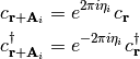
We have a wraparound() (and wraparound_site!, and wraparoundη) function, which takes a site that may or may not be on the actual finite lattice, and returns its lattice index along with the phase that it picks up. So for instance given the site $\mathbf{r}_\alpha + \mathbf{A}_i$ , it returns the site index $\alpha$ of $\mathbf{r}_\alpha$ along with the phase $\eta_i$ picked up when [un]wrapping the boundary conditions. As above, the phase $\eta_i$ returned is defined by

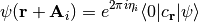
$\psi(\mathbf{r} + \mathbf{A}_i) = e^{2\pi i\eta_i}\psi(\mathbf{r})$

There is also a translation_operators() method, which returns a “translation operator” (really a vector meant for mapping) for each dimension in which $M_{ii}$ is nonzero (i.e. for each direction that is not OBC). So, for instance, translation_operators()[i][alpha] returns the new site index $\beta$ (along with any phase picked up $\eta$ ) of the site $\mathbf{r}_\alpha + \mathbf{a}_i$ such that

$\psi(\mathbf{r}_\alpha + \mathbf{a}_i) = e^{2\pi i\eta}\psi(\mathbf{r}_\beta).$

Wrapping condition in second quantization¶

We wish to generalize the above wrapping equation to second quantization. Note that $\psi(\mathbf{r}) = \langle \mathbf{r} \vert \psi \rangle = \langle 0 \vert c_\mathbf{r} \vert \psi \rangle$ . Using this, we get

$\psi(\mathbf{r} + \mathbf{A}_i) = \langle 0 \vert c_{\mathbf{r} + \mathbf{A}_i} \vert \psi \rangle$

$\psi(\mathbf{r} + \mathbf{A}_i) = e^{2\pi i\eta_i} \langle 0 \vert c_{\mathbf{r}} \vert \psi \rangle$

Together, these imply

$c_{\mathbf{r} + \mathbf{A}_i} &= e^{2\pi i\eta_i} c_{\mathbf{r}} \\ c_{\mathbf{r} + \mathbf{A}_i}^\dagger &= e^{-2\pi i\eta_i} c_{\mathbf{r}}^\dagger$

As a result of this,

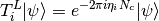
$T_i^L \vert \psi \rangle = e^{-2\pi i\eta_i N_c} \vert \psi \rangle$

when working in second quantization. (Explain this.) where $N_c$ is the “charge” (poorly chosen name, which should be updated.)

API Reference¶

realspace()¶

momentum() function, kdotr¶

nearest_neighbors() functions¶

Returns (via a callback) $i$ , $j$ , and $\eta$ , such that the relevant hopping term would be $e^{2\pi i\eta}c_i^\dagger c_j$ . (FIXME, I have changed this.)

Specific lattice implementations¶

Hypercubic¶

works in any dimension
does not double count bonds on a two-leg ladder (fixme: do we really want this?)
when considering nearest neighbors, do we really want it to be this general? oh well, we can have subclasses that specialize it, since next-nearest neighbors will mean something different depending on dimension.